The Ant System for Problems with Discrete Variables with Beam Design Example

Introduction

The original Ant System (AS) was proposed by Marco Dorigo in 1990. AS has shown its efficiency and simplified concept in solving discrete and combinatorial problems like the Traveling Salesman Problem (TSP), Knapsack, Vehicle Routing, Job Scheduling, for example. Most of the problems to be solved by AS are NP-hard, which are difficult to solve using other meta-heuristic algorithms.

Traveling Salesman Problem solved by ACO (S. Mirjalili, 2018)

AS algorithm is analogous to finding a new cooking recipe where a group of chefs tries to choose the ingredients from the list. The taste of the food is feedback, as an objective value. Each ingredient, like meat, egg, and onion, for example, has a different heuristic and was chosen at different times based on how it could improve the value of the completed food.

Analogy

Chefs	Ants
Each food plate	Each path option, each design solution
Taste	Objective value
Cost of the ingredient	Distance of each individual path, Unit price of each item
Trace of selected ingredient	Pheromone

The pseudo code of the Ant System (AS) is listed below.

Initialize pheromone trails τ(i) = τ0

Set algorithm parameters: α, β, ρ, Q

For iter = 1 to maxIter

    For each ant k = 1 to nAnts

        Construct a solution:

            For each decision variable j

                Compute probabilities:

                   P(option) ∝ τ(option)^α * η(option)^β

                Select option by Roulette Wheel

            End

        Evaluate objective value f(Sk)

    End


    Evaporate pheromone:

        τ(i) = (1 - ρ) * τ(i)

    Reinforce pheromone:

        For each ant k

            For each option chosen in solution Sk

                τ(option) = τ(option) + Q / f(Sk)
        End
    End

    Update best solution

End

Concept

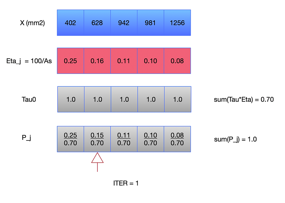
Each ant picks up the design option from the list, which can be one of the items for each list, or the travel path from i to j, based on the probability Pj. Higher probability items get more chances to be selected by the Roulette wheel operation, like in GA. The Probability is built up from the relative pheromone level, i.e.

Pj = Tau_j*Eta_j/sum_all(Tau*Eta) where Tau = Pheromone value = Q/f(x) = Q/Cost

for minimization problem smaller As --> more pheromone then Tau = 100/As

In AS, the total pheromone is computed for each solution from ant 'k' after each iteration

Delta_Tau for ant 'k' is added to the total pheromone only for the chosen solution S_k and zero for others.

Q = scaling factor

Eta = Heuristic i.e. Value of the item j = 1/ Cost_j or 1/Path_distance

In this example, the smaller As is better then Eta = 100/As.

Example -- Concrete Beam Design

We want to design a single-span beam L = 6 m subjected to a uniform load w = 25 kN/m. Then the maximum moment at mid span is Mu = w*L^2/8 = 25*36/8 = 112.5 kNm. Given, fy = 400 MPa, d = 500 mm

The objective is to find the rebar with the minimum weight. The rebar is only available from the list.

Constraint:

0.9xMn > 1.6xMu, where Mn = Asfy(0.9d)

The AS loop can be explained as shown below. In the first iteration, the pheromone is given as 1.0. The rebar with lower weight per length has a higher chance of being selected. However, it turns out that the larger rebar size finally becomes the best solution due to the imposed constraint.

The ACS (Ant Colony System) is the updated version of AS, also by Dorigo (1996). The pheromone (Tau) is updated immediately after each ant 'k' get its solution. So the update is done 'k' time for each iteration. This local update leads to faster convergence as shown in the convergence plot. This is the same manner as used in stochastic gradient descent. Global update after each iteration is done only by the best ant (best solution), same as in AS.

The pseudo code for ACS is shown as following

Initialize pheromone trails τ(i) = τ0

Set algorithm parameters: α, β, ρ, Q, q0, ξ



For iter = 1 to maxIter

    For each ant k = 1 to nAnts

        Construct a solution:

            For each decision variable j

                Compute probabilities:

                   P(option) ∝ τ(option)^α * η(option)^β

                If rand < q0:

                    Select option with highest P (greedy)

                Else:

                    Select option by Roulette Wheel



                Local pheromone update:

                   τ(option) = (1 - ξ)*τ(option) + ξ*τ0

            End

        Evaluate objective value f(Sk)

    End



    Global pheromone update (only best ant):

        Evaporation:

            τ(i) = (1 - ρ) * τ(i)

        Reinforcement:

            For each option in best solution Sbest

                τ(option) = τ(option) + Q / f(Sbest)

    Update best solution

End

What if the number of variables is more than 1?

The same algorithm structure is used, but we just add the loop for each design variable inside the ant loop. Let's see the pseudo-code below.

Initialize pheromone τ(var,option)

For iter = 1:maxIter

   For each ant

       For var = 1:2

          Compute probs for this variable

          Select option (roulette / ACS rule)

          Save choice

          Local update (ACS)

       End

       Evaluate full design (beam1, beam2)

       Save cost, feasibility

   End

   Evaporate pheromone

   Update pheromone deposits (all ants in AS, best ant in ACS)

   Record best solution

End