Comparison of Integration Methods for General Dynamic Response

Introduction

Several time-integration methods for the dynamic response of structures subjected to general time-dependent loading are available. They are classified into 3 main methods: 1. Duhamel's integral (Superposition of impulse)

2. Fourier Series & Fourier Integral (Superposition of the global sine and cosine waves)

3. Direct time integration

Duhamel's Integral

The Duhamel integral transforms the continuous load function into a sequence of discrete impulses. Then the response from each impulse, with a time lag of Tau, is summed to obtain the total response. Obviously, this method is only applied to linear problems.

Superposition of the impulse response by Duhamel's integral

Fourier Series & Fourier Integral

The periodic load function can be decomposed into several simple sine and cosine (harmonic) functions, where the force magnitude can be computed as Fourier coefficients. The total response is the summation of the responses from each of those simple harmonic waves.

The accuracy of using the Fourier series depends on the number of Fourier terms to expand. This method is therefore only applied to linear transient problems with periodic excitation. For a non-periodic load, the more advanced Fourier integral (Fourier Transform) can be applied.

Type of function	Periodic	Non-periodic or transient
Frequency content	Discrete	Continuous
Frequencies	n*omega_0	all omega
Load representation	Sum	Integral
Best for	harmonic/periodic loading	earthquake, impulse, arbitrary time history
Structural response	sum of harmonic steady-state responses	inverse transform of full frequency-domain response

Direct Time Integration Methods

The dynamic equilibrium equation consists of the unknown displacement, velocity, and acceleration at t+1 (the next time step), which can be solved directly by time integration. The word 'direct' means that the equation won't be transformed to any other subspace (i.e. mode shape) before solving (Bathe, 1996).

The direct integration method can be implemented as an implicit or Explicit method. The implicit method, for example, the Newmark method, Taylor's series is used to approximate velocity and acceleration at t + 1 in terms of the solution at time step t. Finally, the unknowns at t+1 are cast into the unknown displacement u(t+1), then solved by a linear system equation, i.e.

[K_eff]{u(t+1)} = F_eff(t)

[K_eff] = [K] + a*[M] + a1*[C] is known and might need to be updated for a nonlinear problem. The RHS force vector is known at time step t, and we can solve the displacement at t+1. Then the velocity and acceleration can be computed using Taylor's expansion formula.

The MATLAB code to perform the solution at time step t+1 is shown below

The explicit methods is based on finite difference approximation of velocity and acceleration in terms of displacement at t+1, i.e.

v(t+1) = (u(t+1)-u(t-1))/2dt. --- (1)

a(t+1) =( v(t+1)-v(t-1))/dt = (u(t+1)-2u(t)+u(t-1))/dt^2 --- (2)

Then

Ma(t+1) + Cv(t+1) + Ku(t+1) = F(t+1) --- (3)

Substituting (1) and (2) into (3) gives

[M/dt^2 + C/2dt] u(t+1) + [K-2M/dt^2] u(t) + [M/dt^2-c/2dt] u(t-1) = F(t)

• Note

  For nonlinear problem, K u(t+1) is replaced by F_int (u_t+1). The equation must the nbe solved using Newton-Raphson iteration

  (see https://www.alpsconsult.net/post/algorithm-template-for-nonlinear-dynamic-solver-using-the-newmark-method for more details)

  
  

Then u(t+1) can be solved for from this equation using the known u(t) and u(t-1). This requires inverting the term [M/dt^2 + C/2dt], but if M and C are diagonal, the elimination process is not needed. The MATLAB code to perform the solution at time step t+1 is shown below

It should be noted that the initial solution u(t-1) is also unknown but can be computed from backward Taylor's approximation (-dt)

u(t-1) = u(t) - v(t)*dt + 1/2 a(t)*dt^2

MATLAB code

The implicit method is unconditionally stable for any dt. It has an advantage in loading that excites low- to moderate-frequency responses, such as seismic loads. However, the time step must still be sufficiently small to ensure accuracy and nonlinear convergence.

The explicit method is conditionally stable. A sufficiently small value of dt is normally necessary; dt < Tn/pi is required for a stable response, where Tn represents the lowest fundamental period of the system. This is suitable for impact and contact problems, such as vehicle crashworthiness analysis and wave propagation. It's not a standard method for seismic response analysis of structures.

Method	Main idea	Best suited for	Load type	System type	Strength	Limitation
Duhamel integral	Response is obtained by convolution of load with impulse response	SDOF / modal linear dynamics	Arbitrary time history	Mainly linear	Very clear physical meaning; exact for linear systems	Less convenient for nonlinear FEM; integral evaluation can be costly
Fourier series	Periodic load is decomposed into discrete harmonic components	Periodic vibration, machine loads, repeated loads	Periodic load	Linear	Elegant frequency-domain solution; shows resonance clearly	Not natural for transient loads unless artificially repeated
Fourier integral / transform	Non-periodic load is decomposed into continuous frequency components	Earthquake, blast, pulse, arbitrary transient load	Non-periodic / transient	Linear	Efficient with FFT; useful for frequency-response analysis	Needs care with sampling, leakage, zero-padding, wrap-around
Newmark method	Marches response step-by-step in time using displacement, velocity, acceleration update formulas	General structural dynamic analysis and FEM	Any sampled time history	Linear and nonlinear	Very practical; works with MDOF FEM; can include material/geometric nonlinearity	Accuracy depends on time step and parameters; nonlinear case needs Newton iteration
Central difference	Explicit time integration using previous/current displacement	Impact, wave propagation, large explicit FEM	Any sampled time history	Linear and nonlinear	Simple and fast per step; no global matrix factorization	Conditionally stable; requires very small time step
Wilson-\theta	Extends acceleration assumption over enlarged time step \theta \Delta t	Linear structural dynamics, older FEM codes	Any sampled time history	Mostly linear	Strong numerical stability	Can introduce numerical damping and phase error

Situation	Recommended method
Closed-form understanding of linear SDOF response	Duhamel integral
Periodic machine vibration	Fourier series
Earthquake record in the frequency domain	Fourier transform / FFT
General FEM time-history analysis	Newmark
Nonlinear frame / material plasticity / geometric nonlinearity	Newmark + Newton iteration
Very fast short-duration impact analysis	Central difference

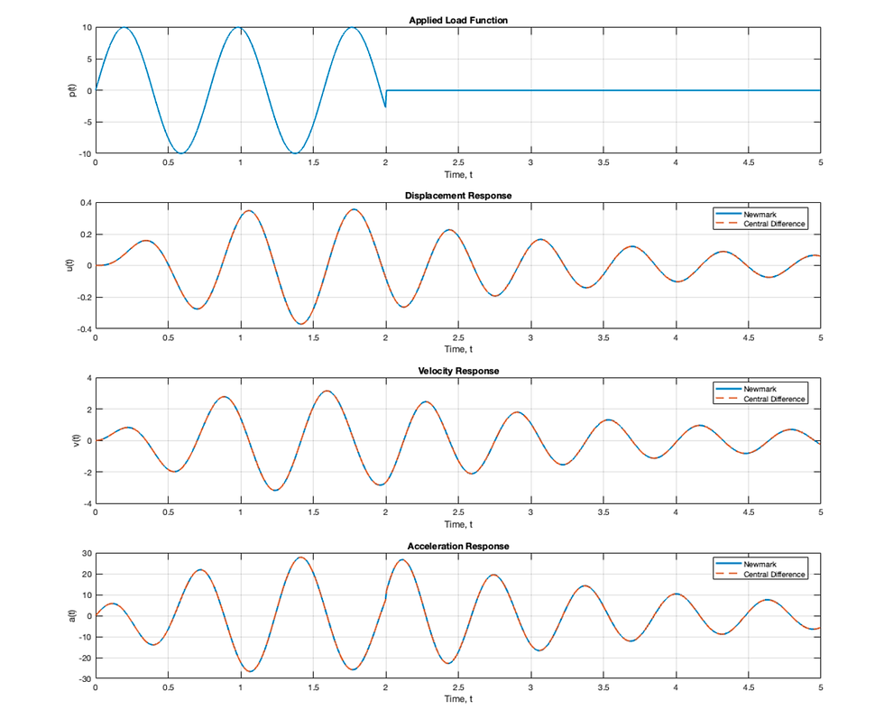
Comparison of Newmark (Implicit) and Central Difference (Explicit) solutions

compare_implicit_explicit.zip

Download ZIP • 2KB

References:

Bathe, Finite Element Procedure, Prentice-Hall, 1996

Cimellaro and Marasco, Introduction to Dynamics of Structures and Earthquake Engineering, Springer, 2018

Oechsner, Computational Statics and Dynamics, Springer, 3rd ed, 2023