Geometric Nonlinear Truss using Updated Lagrangian (UL) – MATLAB Implementation

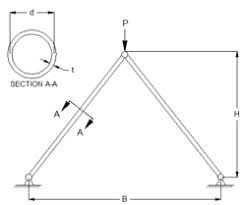
Inclined 2-Bar Truss with Geometric Nonlinearity and Transformation Matrix

This example models a 2-bar inclined truss using the Updated Lagrangian (UL) method. Each bar is inclined, and local stiffness is transformed to global coordinates using a transformation matrix. Geometric stiffness is included in the global stiffness matrix, but element forces are derived only from material strain.

MATLAB Code: Inclined 2-Bar Truss with Transformation

% Properties and Geometry
A = 0.01; E = 200e9; Et = 2e9; sigma_y = 250e6;

coords0 = [0 0; 2 1; 4 0]; % Node 1, 2, 3 (X,Y)

conn = [1 2; 2 3]; % Two truss bars

F_ext = zeros(6,1); F_ext(5) = 0; F_ext(6) = -300e3; % Load at Node 3 (vertical)



% Initialization

u = zeros(6,1); % DOF vector (2 per node)

u_hist = [];



for step = 1:1 % Single load step for simplicity

    f_ext = F_ext;

    u_iter = u;

    for iter = 1:20

        K_global = zeros(6); f_int = zeros(6,1);

        coords = coords0 + reshape(u_iter,2,[])'; % Update node positions



        for e = 1:size(conn,1)

            i = conn(e,1); j = conn(e,2);

            xi = coords(i,:); xj = coords(j,:);

            x0i = coords0(i,:); x0j = coords0(j,:);



            L0 = norm(x0j - x0i);

            Le = norm(xj - xi);

            eps = (Le - L0)/L0;



            % Determine current stiffness

            Ee = (abs(eps*E) < sigma_y) * E + (abs(eps*E) >= sigma_y) * Et;

            N = A * Ee * eps;



            % Local to global transformation

            lx = (xj(1) - xi(1)) / Le;

            ly = (xj(2) - xi(2)) / Le;

            T = [lx ly 0 0; 0 0 lx ly]; % Transform 2D axial to global



            % Local element stiffness matrices

            ke = A * Ee / L0 * [1 -1; -1 1];      % Material stiffness

            kg = N / Le * [1 -1; -1 1];           % Geometric stiffness

            k_local = ke + kg;



            % Global transformation

            K_global_e = T' * k_local * T;



            % Assemble into global matrix

            idx = [2*i-1 2*i 2*j-1 2*j];

            K_global(idx,idx) = K_global(idx,idx) + K_global_e;



            % Internal force (only from axial strain, not geometric stiffness)

            f_local = N * [-1; 1];

            f_global = T' * f_local;

            f_int(idx) = f_int(idx) + f_global;

        end



        r = f_ext - f_int;

        if norm(r) < 1e-3, break; end

        du = K_global \ r;

        u_iter = u_iter + du;

    end



    u = u_iter;

    u_hist = [u_hist, u];

end

🔧 STRUCTURE OVERVIEW:

• 3 Nodes, 2D: Node 1 (fixed), Node 2 (middle), Node 3 (right)

• 2 inclined truss bars: Bar 1 (Node 1–2), Bar 2 (Node 2–3)

• 6 DOFs (2 per node)

• Load applied at Node 3 in the Y-direction

🧠 STEP-BY-STEP EXPLANATION:

✅ 1.

Define Material, Geometry, and Connectivity

A = 0.01;              % Cross-sectional area (m²)
E = 200e9;             % Elastic modulus (Pa)
Et = 2e9;              % Tangent modulus after yield (Pa)
sigma_y = 250e6;       % Yield stress (Pa)

coords0 = [0 0; 2 1; 4 0];  % Undeformed (initial) coordinates (3 nodes, X-Y)
conn = [1 2; 2 3];          % Element connectivity

• Each element connects two nodes.

• The truss is inclined — so transformation is required.

✅ 2.

External Load Vector

F_ext = zeros(6,1);
F_ext(6) = -300e3;  % Apply vertical load at Node 3 (DOF 6)

• Node 3 vertical DOF only.

✅ 3.

Initialization

u = zeros(6,1);     % Nodal displacement vector (6 DOFs)
u_hist = [];        % Store displacement history

• Initially no displacements.

✅ 4.

Outer Load Step Loop (1 step shown for simplicity)

for step = 1:1
    f_ext = F_ext;
    u_iter = u;

✅ 5.

Newton-Raphson Iteration Loop

for iter = 1:20
    K_global = zeros(6);
    f_int = zeros(6,1);

• Initialize residual and global stiffness for this iteration.

✅ 6.

Update Geometry with Current Displacement

coords = coords0 + reshape(u_iter, 2, [])';

• Updated Lagrangian: new geometry at each iteration.

✅ 7.

Loop Through Each Truss Element

for e = 1:2

✅ 8.

Element Geometry and Strain

xi = coords(i,:); xj = coords(j,:);
x0i = coords0(i,:); x0j = coords0(j,:);

L0 = norm(x0j - x0i);   % Original length
Le = norm(xj - xi);     % Current length
eps = (Le - L0)/L0;     % Engineering axial strain

✅ 9.

Determine Effective Modulus

Ee = (abs(eps*E) < sigma_y) * E + (abs(eps*E) >= sigma_y) * Et;
N = A * Ee * eps;       % Axial force

• Bilinear stress-strain model: switch from E to Et at yield.

✅ 10.

Transformation Matrix

lx = (xj(1) - xi(1)) / Le;
ly = (xj(2) - xi(2)) / Le;
T = [lx ly 0 0; 0 0 lx ly];  % Local → Global

• Converts 1D local stiffness and force to 2D global system.

✅ 11.

Local and Geometric Stiffness

ke = A * Ee / L0 * [1 -1; -1 1];  % Material stiffness
kg = N / Le * [1 -1; -1 1];       % Geometric stiffness

✅ 12.

Transform to Global Coordinates

K_global_e = T' * (ke + kg) * T;

✅ 13.

Assemble into Global Stiffness Matrix

idx = [2*i-1 2*i 2*j-1 2*j];
K_global(idx,idx) = K_global(idx,idx) + K_global_e;

✅ 14.

Compute Internal Force from Strain

f_local = N * [-1; 1];         % Axial force vector in local
f_global = T' * f_local;      % Convert to global
f_int(idx) = f_int(idx) + f_global;

💡 No geometric stiffness used in force — only strain-based!

✅ 15.

Solve Residual and Update Displacement

r = f_ext - f_int;
if norm(r) < 1e-3, break; end
du = K_global \ r;
u_iter = u_iter + du;

✅ 16.

Save Final Displacement

u = u_iter;
u_hist = [u_hist, u];

✅ Summary

Feature	Implementation
Geometry update	Yes (UL formulation)
Geometric stiffness	Yes (added to K matrix)
Material nonlinearity	Bilinear model (E, Et, σ_y)
Internal force	Based on strain only (not from k_g)
Transformation matrix	Converts local stiffness to global coordinates
Solver	Newton-Raphson with convergence check