
Stock Market Inspired Optimization
- Adisorn O.
- Sep 27, 2025
- 4 min read

In this post, I introduce a new way of thinking about Swarm Intelligence (SI) algorithms through the analogy of investors and retailers in the stock market. Unlike traditional metaphors that focus on birds, bees, or wolves, this approach models the solutions themselves as “stocks” while investors and retailers represent different search behaviors. Investors are the leaders who identify promising opportunities first, pulling the search toward profitable regions. Retailers follow these leads but apply their own tweaks and randomness, occasionally finding even better opportunities. If the “stocks” turn out to be unprofitable, the system refreshes them—just as in real markets where underperforming assets are abandoned.
This simple analogy translates directly into a population-based metaheuristic:
Exploration comes from retailers experimenting with random tweaks and regenerated stocks.
Exploitation arises from investors steadily pulling solutions toward the best opportunities.
Adaptivity is introduced through simulated annealing–style acceptance, gradually reducing risk over time.
By combining these ingredients, the Investor–Retailer SI provides a flexible and intuitive search mechanism for engineering optimization and other complex design tasks.
Comments on Advantages
Intuitive metaphor
The stock market analogy is widely relatable—readers instantly understand the concepts of “good stocks,” “followers,” and “refreshing portfolios.” This makes the algorithm easier to explain to non-specialists compared to, say, bats or bees.
Balanced exploration–exploitation
Investors ensure convergence by pulling toward the best solutions (exploitation).
Retailers inject diversity by tweaking solutions and occasionally accepting worse moves (exploration).
This dual role naturally balances global and local search.
Adaptive acceptance rule
The simulated annealing–style probability prevents premature convergence in early iterations, while gradually enforcing greediness in later stages.
This mechanism provides robustness against local minima.
Simplicity of implementation
The algorithm uses only a few key parameters (leader pull β, tweak scale σ, and acceptance temperature T).
No complex operators (like crossover, velocity vectors, or harmony memory) are required.
Flexibility for constraints
Since the update rule is general, penalty methods or adaptive constraint handling can be plugged in easily for engineering design problems.
Potential for hybridization
The investor pull resembles PSO’s global best.
The retailer tweak resembles ABC or DE’s differential step.
The acceptance rule resembles SA.
By unifying these, IR-SI can serve as a bridge between major SI families, making it easy to hybridize.
Pseudo Code
Input: Objective function f(x), search space bounds [lb, ub]

Parameters: population size N, max iterations MaxIt

            leader pull β, tweak scale σ0, initial acceptance T0

            refresh rate (fraction of solutions to regenerate), stall limit


1. Initialize population of "stocks" Xi randomly within [lb, ub], i=1…N

2. Evaluate fitness Fi = f(Xi) for all i

3. Identify the best stock X* with fitness F*


4. For t = 1 to MaxIt:

      T = T0 * (1 - t/MaxIt)         // cooling schedule

      σ = σ0 * (1 - t/MaxIt)         // shrinking tweak scale


   For each stock i = 1…N:

      a) Investor move (leader pull):

         Xnew = Xi + β * (X* - Xi)


      b) Retailer tweak (local/random search):

         With probability 0.5:

             Xnew = Xnew + σ * Normal(0,1)

         Else:

             Select random stock k ≠ i

             φ = random(-1,1)

             Xnew = Xnew + φ * (Xi - Xk)


      c) Bound correction: clamp Xnew to [lb, ub]


      d) Evaluate fnew = f(Xnew)


      e) Acceptance rule:

         If fnew ≤ Fi

            Accept: Xi = Xnew, Fi = fnew

         Else if rand < exp(-(fnew - Fi)/T)

            Accept with probability (simulated annealing style)

         Else

            Reject: keep Xi


   End For


   f) Update global best (X*, F*)


   g) If no improvement for "stall limit":

        Refresh a fraction of worst solutions randomly (scout step)


   h) Record best fitness F* for history


End For


Output: Best solution X*, best fitness F*
MATLAB
function [bestx,bestf,history] = IR_SI(obj, lb, ub, opts)

% Investor–Retailer Swarm (ABC+PSO+SA flavor)

% obj: @(x) objective (minimize). lb,ub: row vectors

% opts: struct with fields N, maxIt, beta, sigma0, T0, refreshRate


rng('shuffle');

n  = numel(lb);

N  = getfieldwithdefault(opts,'N',30);

IT = getfieldwithdefault(opts,'maxIt',200);

beta = getfieldwithdefault(opts,'beta',0.6);

sigma0 = getfieldwithdefault(opts,'sigma0',0.2);

T0   = getfieldwithdefault(opts,'T0',0.5);           % SA temperature

refresh = getfieldwithdefault(opts,'refreshRate',0.15); % fraction refreshed if stagnant

stallMax = getfieldwithdefault(opts,'stallMax',20);


X = repmat(lb,N,1) + rand(N,n).*repmat(ub-lb,N,1);

F = arrayfun(@(i)obj(X(i,:)), 1:N).';

[bestf,idx] = min(F); bestx = X(idx,:);

history = zeros(IT,1);

stall = 0;


for t = 1:IT

    T = T0*(1 - t/IT);                    % cooling

    sigma = sigma0*(1 - t/IT);            % shrinking tweak scale


    for i = 1:N

        % --- Investor pull (toward current best) ---

        x = X(i,:) + beta*(bestx - X(i,:));

        % --- Retailer tweak (local/random) ---

        if rand < 0.5

            % Gaussian tweak

            x = x + sigma*randn(1,n).*(ub-lb);

        else

            % ABC-like differential tweak

            k = randi(N); while k==i, k=randi(N); end

            phi = (2*rand(1,n)-1);        % in [-1,1]

            x = x + phi.*(X(i,:) - X(k,:));

        end

        % clamp to bounds

        x = max(min(x,ub),lb);


        fnew = obj(x);

        % --- Accept: improve OR SA probability ---

        if (fnew <= F(i)) || (rand < exp(-(fnew - F(i))/max(T,1e-12)))

            X(i,:) = x; F(i) = fnew;

        end

    end


    % Update global best

    [curf,idx] = min(F);

    if curf < bestf - 1e-12

        bestf = curf; bestx = X(idx,:); stall = 0;

    else

        stall = stall + 1;

    end


    % --- Scout/refresh (regenerate some stocks) ---

    if stall >= stallMax

        m = max(1, round(refresh*N));

        J = randperm(N,m);

        X(J,:) = repmat(lb,m,1) + rand(m,n).*repmat(ub-lb,m,1);

        F(J) = arrayfun(@(k)obj(X(J(k),:)), 1:m).';

        stall = 0;

    end


    history(t) = bestf;

end

end


function v = getfieldwithdefault(s, name, default)

if isfield(s,name), v = s.(name); else, v = default; end

end
Example: Cantilever Beam Design Problem

Minimize f(b,h) = bh
Subject to:
Stress constraint PL/(bh^2/6) < sigma_allow
With P = 10e3 N, σ_allow = 20e5 Pa
% Beam design toy problem
clear; clc;
P = 10e3; % load [N]
L = 5.0; % cantilever span (m)
sig_allow = 20e5; % [Pa]
obj = @(x) cost_fun(x,P,sig_allow,L);
lb = [0.1 0.1]; % b,h lower bounds [m]
ub = [2.0 2.0]; % upper bounds
opts.N = 5; opts.maxIt = 100;
opts.beta = 0.7; opts.sigma0 = 0.2; opts.T0 = 0.5;
[bestx,bestf,history] = IR_SI(obj,lb,ub,opts);
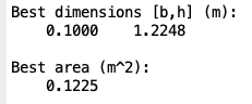
disp('Best dimensions [b,h] (m):'); disp(bestx);
disp('Best area (m^2):'); disp(bestf);
figure; plot(history,'LineWidth',2);
xlabel('Iteration'); ylabel('Best Area');
title('Investor–Retailer SI: Beam Design Problem');
grid on;
% ----- helper function -----
function f = cost_fun(x,P,sig_allow,L)
b = x(1); h = x(2);
area = b*h;
modulus = b*h^2/6;
stress = P*L/modulus;
if stress > sig_allow
penalty = 1e6*(stress/sig_allow - 1); % simple penalty
else
penalty = 0;
end
f = area + penalty;
end

Reference:
Adisorn Owatsiriwong (2025). Stock Market Inspired Optimization (https://www.mathworks.com/matlabcentral/fileexchange/182147-stock-market-inspired-optimization), MATLAB Central File Exchange. Retrieved September 27, 2025.