
Underground Water Tank Analysis and Design using Reissner-Mindlin Plate Elements
- Adisorn O.
- May 20
- 4 min read

Updated: Jun 16
Adisorn Owatsiriwong
ALPS Consultants
Introduction

An underground water tank’s wall is a 2D structure that requires detailed analysis using design charts or sophisticated FEM modeling, e.g., SAP2000. This time-consuming process requires a structural engineer to model the tank geometry and provide triangular load definitions to the model.
In this project, we use the Reisner-Mindlin plate element (Bathe, 1996; Bishoff, 2002) to develop a handy FEM tool for water tank analysis and design. The model can simulate a triangular pressure profile using simple input parameters. It's applied to soil and water pressure. Along the boundary lines, both free and fixed support conditions can apply to the node. After the design moments are obtained using Armer-Wood's equation, the rebar quantities in the X and Y directions are computed using the ACI 318-19 approach. The shear stress X and Y are also computed from Qx/t and Qy/t in kPa to compare with the reduced concrete shear strength.
The FEM code is developed on MATLAB using 4-node quads with isoparametric shape functions. The following formulation is followed.
Strain-displacement relations

Constitutive matrices
The stress resultants M (bending moment/unit length) and Q (transverse shear force/ unit length) is related to the strain vector as following:

The constitutive matrix was derived from plane stress (in-plane) condition i.e.,

Notation:
Mx is a bending moment to bend the plate in local +x axis, and My is a bending moment to bend in +y local axis. Positive Mx, My will cause +z surface to be in tension, i.e., see the definition of curvature in section 2. This is a standard notation used in our software tools.
Four-node Q4 R-M plate element
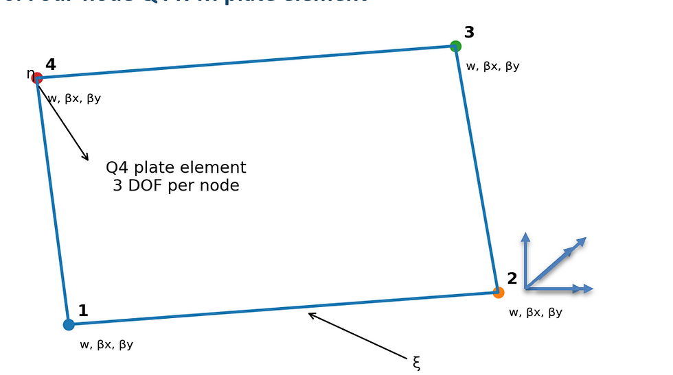
Figure 2. Four-node R-M plate element with three DOF per node: w, βx, βy.
For a four-node isoparametric quadrilateral element, the nodal displacement vector is ordered as:
de = [w1 βx1 βy1 w2 βx2 βy2 w3 βx3 βy3 w4 βx4 βy4]ᵀ
The bilinear shape functions in the natural coordinates ξ, η are:
N1 = 1/4(1-ξ)(1-η), N2 = 1/4(1+ξ)(1-η)N3 = 1/4(1+ξ)(1+η), N4 = 1/4(1-ξ)(1+η)
The field variables are interpolated from nodal values:
w = Σ Ni wiβx = Σ Ni βxiβy = Σ Ni βyi
The bending strain-displacement matrix Bb contains derivatives of rotation shape functions. The shear strain-displacement matrix Bs contains derivatives of w plus the rotation interpolation.
κx = Σ (∂Ni/∂x) βxiκy = Σ (∂Ni/∂y) βyiκxy = Σ (∂Ni/∂y) βxi + Σ (∂Ni/∂x) βyi
γxz = Σ (∂Ni/∂x) wi + Σ Ni βxiγyz = Σ (∂Ni/∂y) wi + Σ Ni βyi
Stiffness Matrices & Weak Formulation
The finite element formulation is most conveniently derived from the principle of virtual work. For a transverse pressure p(x,y), the internal virtual work equals the external virtual work:
∫A [δκᵀ M + δγᵀ Q] dA = ∫A δw p dA + boundary work
Substituting the constitutive laws gives the element stiffness expression used in the code:
Ke = ∫Ae (Bbᵀ Db Bb + Bsᵀ Ds Bs) dA
The consistent element load vector for transverse pressure is:
fe = ∫Ae Nwᵀ p(x,y) dA
where Nw contains the displacement interpolation functions associated with nodal w DOFs only. If pressure varies linearly with height, the same Gauss integration used for the element can evaluate p at each integration point.
6. Numerical integration and shear locking
A standard Q4 R-M element may suffer shear locking when t/L is small. The element over-constrains transverse shear strains and becomes artificially stiff, causing underpredicted deflection and distorted moments.
· Bending term: usually integrate with 2x2 Gauss points for Q4 elements.
· Shear term: often integrate with 1x1 reduced integration or selective reduced integration to mitigate locking.
· Very distorted meshes can still degrade accuracy; mesh quality matters for plate bending.
· For thin walls, compare against strip solutions, classical plate coefficients, or mesh refinement studies.
Ke ≈ Σgp Bbᵀ Db Bb |J| wgp + Σgp,s Bsᵀ Ds Bs |J| wgp,s
Reduced shear integration is an engineering compromise: it improves thin-plate behavior but can introduce hourglass-like zero-energy modes in some formulations. In practical wall-panel models with sufficient boundary constraints and regular meshes, selective reduced integration is commonly acceptable for first-version tools.
7. Water and soil pressure loading

Figure 3. Hydrostatic pressure field for water height h less than or equal to wall height H.
For a vertical wall coordinate y measured upward from the base and water height h, hydrostatic pressure is:
pwater(y) = γw max(h - y, 0)
For construction-stage soil pressure using an active earth pressure coefficient Ka and retained soil height Hs, the triangular pressure can be represented similarly:
psoil(y) = Ka γsoil max(Hs - y, 0)
The sign of pressure must match the positive transverse direction of the plate DOF w. For two analysis stages, the same FEM kernel can be reused with a different pressure function and different edge support conditions.
8. Boundary conditions for tank wall stages
A practical wall model uses edge restraints to approximate the construction and service-stage boundary conditions. Typical options are:
Edge model | DOF constraint | Physical meaning |
Free | none | No displacement or rotation restraint. |
Simply supported | w = 0; rotations free | Transverse displacement restrained, bending restraint released. |
Clamped / fixed | w = 0, βx = 0, βy = 0 or relevant edge rotation restraint | Edge connected monolithically to stiff slab/wall. |
Symmetry | normal slope/rotation and compatible displacement constraints | Used for symmetric submodels. |
For the user workflow: construction stage may be idealized as a three-side-supported plate with open top; after cover slab construction, the wall can be idealized as four-side-supported. Real restraint stiffness is intermediate, so sensitivity checking is recommended.
Numerical Example

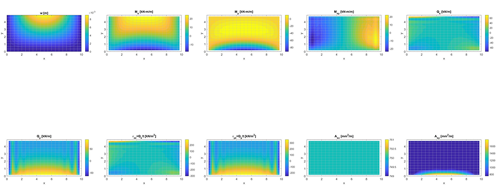
Contour plots of the FEA results

Reference
M Bischoff, Advanced Finite Element Method, Lecture notes at Technische Universität München, 2002
KJ Bathe, Finite Element Procedures, Prentice-Hall, 1996